Spectrum Full Fine Tuning
Spectrum is a new method for full fine-tuning pre-trained language models. It is an approach for efficient LLM fine-tuning that selectively tunes only a small subset of layers based on their SNR (Signal to Noise Ratio).
It Uses Random Matrix Theory (RMT) especially Marchenko-Pastur Law to predict the SNR of each layer. This law charecterizes eigan value distributions in large random matrices.
To understand this better, let’s first understand the basics of Linear Algebra.
Singular Value Decomposition (SVD)
Singular Value Decomposition (SVD) is a matrix factorization technique that decomposes a matrix into three other matrices. It is represented as:
\[\begin{align} W = U \Sigma V^T \end{align}\]
- \(W\) is the input matrix
- \(U\) is an orthogonal matrix
- \(\Sigma\) is a diagonal matrix containing the singular values (\(\sigma_i\)) of \(W\)
- \(V^T\) is the transpose of an orthogonal matrix \(V\)
When applied to the weight matrix of neural networks,
- It helps us identify the most important patterns in the weight matrix by looking at the largest singular values (dominant patterns/directions in weight matrix). Least important patterns (noise) are represented by smaller singular values.
- It can help us understand the underlying structure of the model’s weights and potentially identify which parts of the model are most important.
- Removing the smallest singular values (noise) might suppress factual knowledge or impact the learning of more complex patterns, which can lead to catastrophic forgetting.
Eigan Value Decomposition (EVD)
Eigan Value Decomposition (EVD) is a matrix factorization technique that decomposes a matrix into two matrices. It is similar to SVD but for square matrices. It is represented as:
\[\begin{align} W = Q \Lambda Q^T \end{align}\]
- \(W\) is the input matrix
- \(Q\) is an orthogonal matrix
- \(\Lambda\) is a diagonal matrix containing the eigan values (\(\lambda_i\)) of \(W\)
Relation between SVD and EVD
SVD of a matrix \(W\) of shape \((m \times n)\) is given as \(W = U \Sigma V^T\)
lets look at \(W.W^T\)
\[\begin{align} W.W^T = (U \Sigma V^T)(U \Sigma V^T)^T = U \Sigma^2 U^T \end{align}\]
\(W.W^T\) is a square matrix and can be decomposed using EVD as \(W.W^T = Q \Lambda Q^T\)
so \(\Lambda_{W.W^T} = \Sigma^2_{W}\)
Marchenko-Pastur Law
In random matrix theory, the Marchenko-Pastur Law describes the asymptotic behavior of the eigenvalues of large random matrices. It tells that, For a matrix \(W\) of shape \((m \times n)\) with \(m \geq n\), the eigenvalues of \(\frac{1}{n}W.W^T\) converge to a distribution bounded by:
\[\begin{align} \lambda \in \left[\sigma^2 \left(1 - \sqrt{\frac{m}{n}}\right)^2, \sigma^2 \left(1 + \sqrt{\frac{m}{n}}\right)^2\right] \end{align}\]
the bound for singular values of \(W\) is given by:
\[\begin{align} \sigma \in \left[ \frac{1}{\sqrt{n}} \sigma \left(1 - \sqrt{\frac{m}{n}}\right) , \frac{1}{\sqrt{n}} \sigma \left(1 + \sqrt{\frac{m}{n}}\right)\right] \end{align}\]
Signal to Noise Ratio (SNR)
from above, maximum threshold for the singular value random matrix is \(\sigma_{\text{thresh}} = \sigma \left(1 - \sqrt{\frac{m}{n}}\right)\)
- Removing normalization factor \(\frac{1}{\sqrt{n}}\) to ensure numerical stability.
- Calculating \(\sigma\) using IQR instead of std to account for potential skewness and kurtosis.
lets take \(S\) contains the singular values of \(W\), then SNR is given by:
\[\begin{align} SNR = \frac{\text{count of singular values in S} \gt \sigma_{thresh}}{\text{count of singular values in S} \leq \sigma_{thresh}} \end{align}\]
- normalizing SNR by the largest singular value $ $ for sensitivity analysis, enhanced comparison
- Matrices with higher SNR contain more informative features and less noise.
Layer Selection
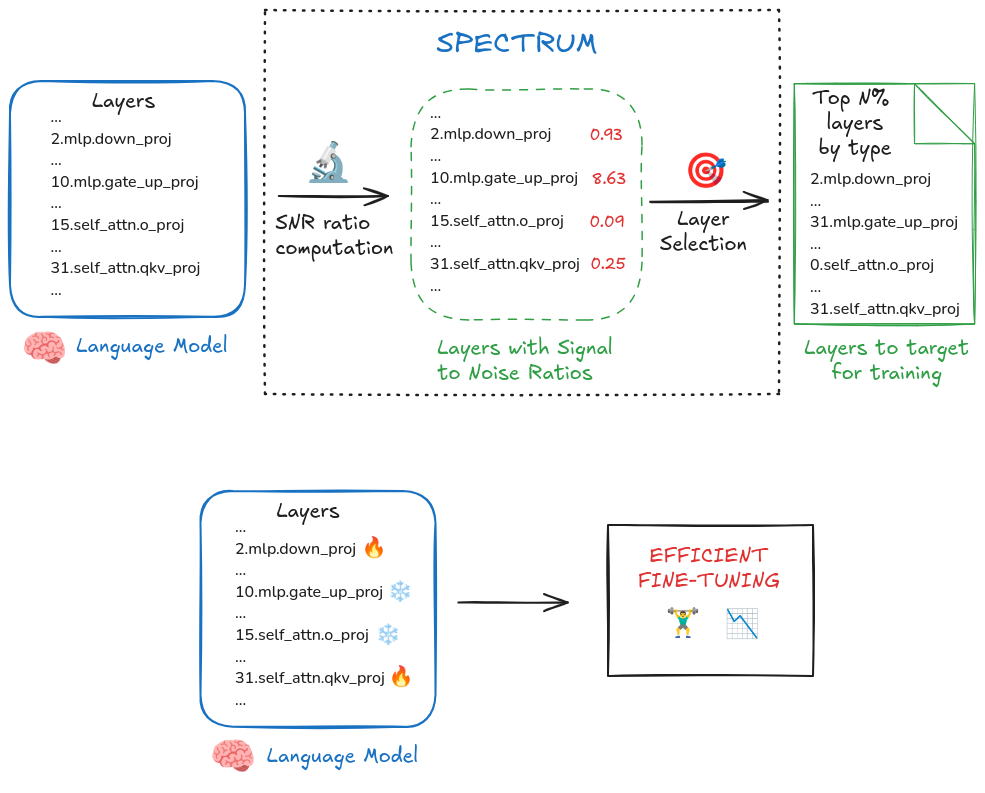
- For each layer, calculate SVD of weight matrix \(W\) and then calculate SNR and normalize it.
- select top \(k\%\) layers with highest SNR.
Kis a hyperparameter.
Reference: 1. https://arxiv.org/abs/2406.06623 2. https://huggingface.co/blog/anakin87/spectrum